- Packages I will use to read in and plot the data
- Read the data in from part 1
Interactive graph
- Start with the data
- Rename the columns
- Reformat the data for r plotting
- Use e_charts to create an e_charts object with description -Use e-bar to build “n” that contain regional deaths by region. The depth of each column represents the amount of deaths for substance abuse disorder
- Use e_tooltip to add a tooltip that will display based on the axis values -Use e_title to add a title
regional_deaths %>%
  rename(drug_use=1,alcohol_disorders=2, illicit_drug=4) %>%
  pivot_longer(cols = 1:5, names_to = "description", values_to = "n") %>%
  arrange(n) %>%
  e_charts(description) %>%
  e_bar(n,legend=FALSE) %>%
  e_flip_coords() %>%
  e_tooltip(trigger = "axis") %>%
  e_title(text = "Annual regional deaths, by world region")
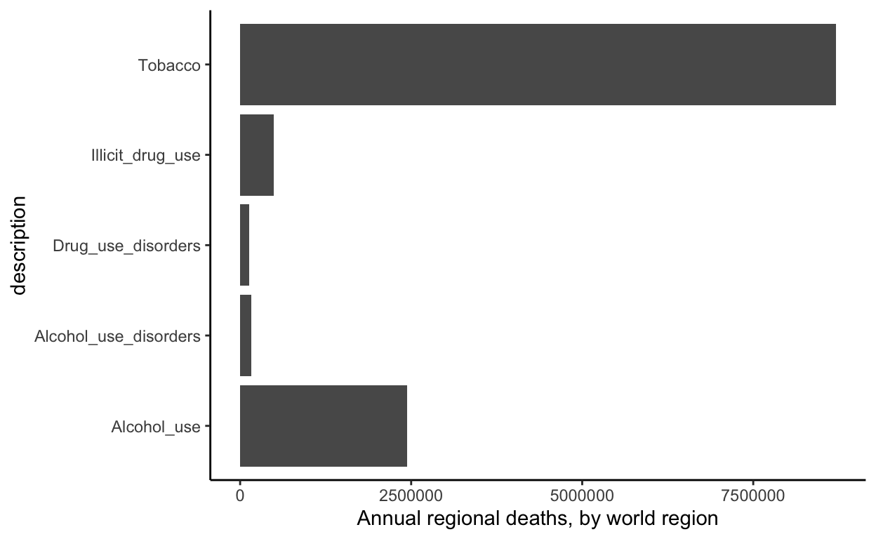
Static graph
- Start with the data
- Use ggplot to create a new ggplot object. Use aes to indicate that description will be mapped to the x axis; n will be mapped to the y axis;
- geom_col will display Regional Deaths
- theme_classic sets the theme
- Theme(legend.position = “bottom”) puts the legend at the bottom of the plot
- labs sets the y Annual regional deaths, by world region
regional_deaths   %>%
  pivot_longer(cols = 1:5, names_to = "description", values_to = "n") %>%
  ggplot(aes(x = description, y = n))+
 geom_col() +
  coord_flip()+
  theme_classic() +
  theme(legend.position = "bottom") +
  labs( y = "Annual regional deaths, by world region")
These plots show a steady increase in deaths since 1900. deaths have continued to increase.